I would say that SPM math is a pretty poor indicator of how good your math skills are, as it promotes rote memorization instead of understanding. Good unis will probably try to let you understand concepts. Like my first year in uni, it completely blew my mind on how mathematics really was.

A good understanding of Math is required to READ several highly theoretical engineering books. When it comes to design, engineers apply the principle and let the computer solve it. Now, let's do a little test and see to what extent you can understand it. Only a small portion of simple SPM/STPM Math is required. The rest is theoretical logic.

When engineers are to improve the design of a system, or to design a new system, a performance index must be chosen and measured. A system is considered an optimal system when the system parameters are adjusted so that the performance index reaches an extremum, commonly a minimum value. The purpose of design is to realize a system with practical components that will provide the desired time-domain operating performance, x(t), with minimal error. In many designs, we are also concerned with the expenditure of the control action/energy, u(t). For example, in electric vehicles and aircraft, the expenditure of battery energy and fuel and must be restricted to conserve the energy for long periods of travel.

Our goal is to find an optimal control u* that minimizes the following performance index (a.k.a. cost function):



where t is the initial time, T is the terminating time, x = x(t) is the current performance state, and L(x,u) characterizes the cost objective.

The Principle of Optimality states, if a control u* is optimal from some initial state, then it must satisfy the following property: after any initial period, the control u* for the remaining period must also be optimal with regard to the state resulting from the control of the initial period.

Now let us consider the current time t and a future time t+Δt closed to t and the control during the interval [t, t+Δt]. Clearly, we can rewrite J(x,t) as



Let J* denote the optimal (minimum) cost under optimal control action u*, then by applying the principle of optimality, we have



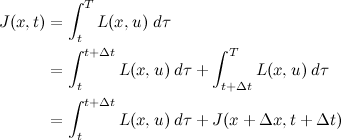
In the above equation, the first term, ∫ L(x,u) dτ can be approximated as , and the second term, J*(x+Δx, t+Δt) can be approximated by its first-order Taylor expansion:



where O(Δt²) denotes the remainder high-order terms (H.O.T.) in the Taylor expansion, which can be omitted if Δt → 0.

Therefore,



Since J*(x,t) and (∂J*/∂t) Δt are independent of u(τ) @ interval [t, t+Δt], the above equation can be written as



Rearranging the equation gives



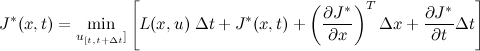
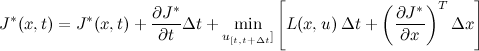
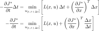
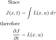
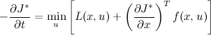
Letting Δt → 0, then . Therefore, we obtain the following Hamilton–Jacobi–Bellman equation:



This post has been edited by Critical_Fallacy: Mar 26 2014, 03:37 PM

Firstly, really thanks so much for your effort !!!!

All the symbols are making me confused .. but I still can understand some of it .. This derivation looks like Differential Equation in STPM

By the way, I was actually worrying about my friend. His Physics is really good, but his maths is just so-so. He has improved a lot in STPM compared to his SPM .. Hoping that he can cope with it if he is to choose Engineering

Just like the first time you were introduced to x, y, z in geometry and f(x), g(y), h(z) in functions. Once you get used to the math symbols, its not so terrible. Not all engineering books are written in such readable manner. Some authors assume the engineering students have adequate knowledge and backgrounds in Math and Calculus, and so they present only the Performance Index J(x,u), and the Hamilton–Jacobi–Bellman equation. And you'll have no idea how they are related to each other. Some students would argue weakly that,



which is erroneous. Therefore, like I emphasized in previous post, a good understanding of Math is required to READ engineering books. And you must NOT refer to only one book but several, so that you can evaluate and select the authors that suit your taste. Are you into medical or engineering?

Really have to take time to comprehend the symbols ..

Yeah, one book is not enough, learned this in STPM

I'm not into both, but will prefer engineering as I'm good(not sure whether I like) in Maths and like Physics(discovered this when SPM is just around the corner)

Anyway, I've chosen my path though, I'm going for Liberal Arts

let see.... SPM maths u can do by understanding it... but engineering maths its kinda like history only this time with numbers and symbols.

Since most of the lecturer will only giv u the theory without letting u know what it is used for. Unless u are lucky and got the good ones....

hi ther, i am engineering student from mmu 3rd year....hehe

Can anyone assist me ? Which colleges have material engineering ?

Engineering Diploma holders of the School are exempted from relevant papers in the BEM/IEM Examination, what does this mean?

Meaning that, students do not need to take this examination from that school.
The reason maybe you will continue the study for degree, and the degree is accredited by BEM.

partially agree with this.
Lecturer in general (especially those in Malaysia, no offense) suck

And regarding engineering maths.. I take it like a more advanced STPM maths. You can opt to fully understand, and do some practices in order to master engineering maths, or you can take the harder way - kind of 'memorize' the methods to do them.

Physics and Engineering Maths (Calculus) are particularly required to model the system dynamics in Differential Equations. Because most high-order, nonlinear Partial DEs do not have closed-form solutions, the analysis are usually performed using advanced computational and numerical methods.

for the math skills thing u dun actually need it when in industrial...

what happens if i went for an engineering institution which is not accredited by BEM? eg.TARC

EAC accreditation is to ensure that graduates of the accredited engineering programmes
satisfy the minimum academic requirements for registration as a graduate engineer with the
Board of Engineers Malaysia (BEM) and for admission to graduate membership of IEM.

<<what happens if i went for an engineering institution which is not accredited by BEM?>>
You not able to register professional engineer (Ir title) in BEM.
Your career will be limited to normal engineering. You don't have career advancement in engineering to Ir.

thx

It depends on the engineering industry and the kind of technical position one takes. Most design and analysis are implemented on a computer for processing speed. Sometimes, however, it is useful as well as a rule of thumb to be able to conduct the simple math computation manually with a few parameter variations to check the validity of the computer programs, or to verify the logic of the analytical results.

In machine we trust, maybe, but not each other as human error has been cited as a primary cause or contributing factor in disasters and accidents in industries as diverse as nuclear power (e.g., Three Mile Island accident), aviation (e.g. Eastern Air Lines Flight 401 crash), space exploration (e.g., Space Shuttle Challenger Disaster and Space Shuttle Columbia disaster), and medical malpractice.

hey i just finished my SPM and i've got fairly good results.. im keen on taking mechanical engineering. may i get suggestions on where i should further my studies and why?

Hi,

Having a degree in engineering is really in demand. But experience is more important, if your looking for better future i would suggest find a stable job first, have the feel of doing the hands on engineering and educational advancement is for position level up and can be done after having enough skills on your kind of field.

For further advise lets talk - pm me .

Did you just replied my post 4 years ago? Interesting to look back what I wrote 4 years back.