Haha, now I kena pusing-pusing by you liao.

But how you update the preset sequence (parameters??) adjusting to current market condition?
i.e. if market X is considered high risk in your program in year 2011, the same might not apply now / in the future.

Add in System Analyst

Released v1.4, can be downloaded via clicking here. This will be the last major update for a while (except critical bug fixes)

Change log:
p/s: as usual, let me know if spotted any errors ya
p/s#2: If you're already existing user of v1.3, there's no "fully automate" way to copy&paste into new template; but what you can do is, utilize the "uber-many-rows-fund" i have prepared in new template; copy those fund values (i.e. all those Negative Transaction Amounts for Fund A) and paste it in those detail rows , then copy the date and paste, and SC% then paste, then manual adjustment then paste.. (MAKE SURE YOU PASTE AS VALUES ONLY!!!!!)
i know it's quite anal for each and every update you'll have to re-enter the details
But I'm looking into how to improve mass-copy-paste data from FSM so less works are required (although you'll still need some basic works to PREPARE the placeholders and create enough rows to "hold" those values....)


KNOWN BUG (minor): In subtotal's line, check the date, make sure it's showing today's date with the formula


Some of the rows have wrong fixed date (i.e. 2014) which may give you some wrong IRR values (was doing some IRR testing, forgot to change it back).

I've updated the version in dropbox to rectify it.

This post has been edited by polarzbearz: Jan 28 2015, 12:10 AM

If you want to do a mass-copy, just make sure that:

1) You only copy & paste values inside (when pasting, choose "Paste Values" only - this will avoid overriding of formats / etc)
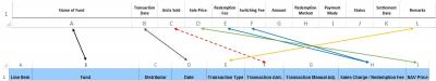
2) Only modify those cells in White Colour / Gold Colour. Dark Grey and Light Grey are ALL formulas (or used in formula)
3) When performing mass-copy-and-paste, make sure there are "enough" rows to hold your paste. If your going to copy 100 rows worth of data for "Date", make sure there are 100 details row for that fund (in my template) to "hold" it.
4) Copy multiple rows' worth of data, one type at a time
----- (e.g. first mass copy all Transaction Dates, make sure it pastes correctly and works;
----- then repeat it for transaction type (most if not all of it has same text with FSM, except some like "Platform Fee Switch Sell", just check before you paste.;
----- then repeat it for Transaction Amount. However, in FSM, its data are formatted as TEXT in "RM XXXX.XX" format. I have a formula to convert this into XXXX.XX format, and you can convert it into NUMBERS, then do a simple NUMBER*-1 to get the negative value, which you can COPY it and PASTE it to my worksheet (PASTE IT AS VALUES ONLY PLEASE!) But use it only if you are comfortable with manipulating excel data (and also please do this in new sheet ). Here's the formula:


----- then repeat it for Sales Charge / RF %, this one pretty straight forward
----- and finally the bread and butter of unit trust, copy the NAV price and paste it (also make sure paste as value & format is accurate).


As for those already-existing data, you can select the entire rows (of that fund) and "Delete Row". (p/s: this is especially important for the "retired" rows, make sure you delete them instead of setting value to 0 as this will screw up IRR formula)

This post has been edited by polarzbearz: Jan 28 2015, 12:23 AM

1. this was the issue previously reported by you where entering "adjustment" at subtotal line does not have effect on the number of calculated units (at subtotal line). now, entering -0.01 at manual adjustment in subtotal line will deduct 0.01 units at subtotal line.

2. previously, manual adjustment works only for "Buy / Switch Buy" where it will adjust the number of units based on your input (i.e. entering -0.01 will minus 0.01 from Calculated Units)
now, manual adjustment also works for "Sell / Switch Sell" where it will adjust the calculated price amount based on your input (i.e. entering -0.01 will minus 0.01 from Amount in RM)

3. I don't think you can copy the new formula and paste it into v1.3 worksheet, as there are a few changes to the column field name. If you are comfortable with it, you can save a backup copy of your v1.3 and try to paste the new formula into it, and in the worksheet, change the header column "SC / RF / MF" into "Sales Charge / Redemption Fee". It should work (backup first to be safe)

Sorry if this is stupid question

Are CMF as safe as Fixed Deposit? Or CMF is still "subject to" market risk but way lower risk than bond / equity?

I see! That sums it up

Managed to get started (recently) thanks to the guys(girls) in this thread

I when I entered the ILP into my portfolio spreadsheet. The sales charge (first few years) exceeded my data validation (between 0% - 100%) and I had to change the data validation

Feel so wasted looking at the ILP but must buy to safeguard my family on the first property

Hopefully it's not a wrong decision, especially after frequenting FSM thread

Investment Linked Policy for Insurance

I tried comparing the term insurance vs. ILP; term insurance's commitment comes up at a bout 40% higher premium per annum for the same TPD&Death coverage, insured at the loan amount.

Then after looking at my commitments, the ILP seems to be more affordable although it carry risks (of non performing market). But the fund I chosen is 50% FI 50% EQ.

This post has been edited by polarzbearz: Jan 31 2015, 11:34 AM

Surprisingly there are very MINIMUM amount of guaranteed cash value.

The product I was quoted for term insurance was this: https://www.aia.net.my/products/main/brochu...30529_final.pdf

should be OK gua, as my main goal of that insurance is to insure the property loan amount for my family, in case anything *choi* happen to me. I choose the lowest possible ILP plan liao, after knowing the initial sales charge etc.

I checked the detailed table, seems to be OK tho.

The insurance charges only take up about 30% of yearly premium paid, should have enough "buffer" to tank during bad market conditions.

Sifus-sifus sekalian,

Currently I'm working on the data importer (converts FSM historic transaction into my spreadsheet format) and as you all know, I'm pretty new to FSM platform and thus, limited amount of data.

Appreciate if any of you (with mass amount of transactions) to share with me the "Transaction Types" available in your "Historic Transactions @ FSM" (not your data. but small sample of your data is appreciated too for testing, if you don't mind ) available in FSM? Currently this is what I'm aware and confirmed of based on my historic transaction + the sample data sent by jutamind for analysis:

For PURCHASES

• Buy
• Switch Buy
• [GUESSING] I'm guessing there's nothing else here. Or maybe Dividend with gained units at zero cost in RM?

For SALES

• Switch Sell
• Platform Fee Sell (<<<< basically equivalent to "Sell" in my spreadsheet)]
• [GUESSING] I'm guessing there will be Sell

Appreciate if any of you could provide inputs as I need to know "Remarks" available in FSM to convert / map it to the "Transaction Type" in the spreadsheet

This post has been edited by polarzbearz: Feb 1 2015, 01:16 PM

But how about the "words" used in FSM Historic Data? As I need the "exact terms" from FSM perspective to do the mapping (i.e. "Sell" in FSM = "Sell" in spreadsheet; "Platform Fee Sell" in FSM = "Sell" in spreadsheet; etc...)

(see the highlighted box above)

Thank you everyone (and anonymous) who have contributed.

I've gathered the list of FSM terminology for Purchase / Sales Historical Data and currently are as follows:-

PURCHASE
Buy
Switch Buy
Dividend
Switch Buy Intra
Unit Split
Transfer In


SALES
Switch Sell
Switch Sell Intra
Sell
Platform Fee Sell

My mapping table will be as follows

SCOPE	FSM TERMINOLOGY	SPREADSHEET TERMINOLOGY	Existing in v1.4?
PURCHASE	Buy	Buy	Yes
PURCHASE	Switch Buy	Switch Buy	Yes
PURCHASE	Dividend	Dividend	Yes
PURCHASE	Switch Buy Intra	Switch Buy	Yes
PURCHASE	Unit Split	Unit Split	No. To be added in v1.5. But seems to have same expected behaviour with Dividends. Not sure to create new type; or tumpang existing?
PURCHASE	Transfer In	STILL THINKING	Seems to have same behaviour with Dividend / Unit Split. Not sure to create new type; or tumpang existing?
SALES	Sell	Sell	Yes
SALES	Switch Sell	Switch Sell	Yes
SALES	Switch Sell Intra	Switch Sell	Yes
SALES	Platform Fee Sell	Sell	Yes
OTHERS	??????????????	Platform Fee	Yes

Will share with everyone once I have completed the import-conversion tool

Anyone have bond funds and charged "Platform Fee"? May I know what is it shown in FSM historic data (under "Remarks" column)

This post has been edited by polarzbearz: Feb 1 2015, 10:22 PM

Pink Spider

I noticed that in "FSM Sales Transaction" there are two types of fees - "Redemption Fee" and "Switching Fee". Is it ok to sum these percentages together?

Example: when selling fund A, it costs me 1% redemption fee and 1.5% switching fee. Can I assume that the total % incurred during this sales transaction is 2.5%? I did a quick test in the excel spreadsheet and seems like the value is the same.

unker yklooi lied to me with his song



Anyway I think it should be OK, I rechecked the formula's + your explanation previously:

Based on the above formula, mathematically speaking it should be correct

But best if anyone has FSM data with "Sales Transaction" which incurs BOTH "Switching Fee" and "Redemption Fee" can share that snippet (just that part) of the data, then I / Pink can do the reverse calculation

Cause I'm just worried that FSM calculates it differently, like [(unit x nav price) * (1 - redemption fee) * (1 - switching fee)] which will end up as RM9751.5 instead of RM9750.00

But for now (without any sample data on above scenario), I'll just proceed to build the tool under the assumption that "redemption & switching fee % are summed together"

This post has been edited by polarzbearz: Feb 2 2015, 11:40 AM

After going through 105++ rows of sample data (related to CMF Sales) and cross-checking excel spreadsheet, I just realized that FSM is not even consistent in their own formula.

Most of the time they round to NEAREST, but sometimes they round down (2 transactions out of 105++ rows)


One extracted example below:

FSM's Calculated Amount	Without Rounding in Excel	With Rounding to 2 decimals in Excel	Type?
RM20,000.00	RM20,000.006165	RM20,000.01	Round down??? NOT OK!

Although RM0.01 is nothing to shout about, but it gave me a heart attack during my troubleshooting when I compared values between FSM (sample) data vs. the spreadsheet . Ingat ada lagi formula salah

Everyone's enjoying our long weekends huh

All the girls talk aside, a little bit of off topic technical post here as usual

I've completed the development of the conversion tool and tested it a few rounds, and I think it should be ready-to-go.

----------------------
Released v1.5 for the Spreadsheet, can be downloaded via clicking here. This will really be the last major update for a while (it's just to accommodate a few new Transaction Types after discovering it through long list of FSM data)

Change log:



p/s: as usual, let me know if spotted any errors ya

----------------------
And also released v1.0 of the Conversion Tool, can be downloaded via clicking here. Please make sure you carefully read the instructions ya, it may look complicated but once you understand how it works (through the Instructions), you should be able to easily convert FSM data into format which can easily be copied-and-pasted into my template (make sure you paste as VALUE only; otherwise formatting will definitely go haywire).

Change log:

As for Pink Spider, need your help to do a one-time update in the first post . I've made changes accordingly (based on your existing first post) in below code so you can just copy&paste easily



Preview